yahoofinancer Cookbook: 15 Practical Recipes • yahoofinancer

Overview

The yahoofinancer package provides a tidyverse-first, type-stable interface for querying market data from Yahoo Finance. This cookbook compiles 15 end-to-end recipes ranging from baseline data extraction to technical indicators, quantitative modeling, risk management, and portfolio performance analysis.

Required Packages

library(yahoofinancer)
library(dplyr)
library(tidyr)
library(ggplot2)
library(scales)
library(zoo)

1. Download Historical Equity Prices

Retrieve daily Open, High, Low, Close, Adjusted Close, and Volume (OHLCV) price series for a single security using either functional or object-oriented (R6) interfaces.

# Functional API
aapl_prices <- yf_download_prices(
  tickers  = "AAPL",
  period   = "1y",
  interval = "1d"
)

head(aapl_prices)
#> # A tibble: 6 × 8
#>   symbol date                 open  high   low close adj_close
#>   <chr>  <dttm>              <dbl> <dbl> <dbl> <dbl>     <dbl>
#> 1 AAPL   2025-08-18 13:30:00  232.  233.  230.  231.      230.
#> 2 AAPL   2025-08-19 13:30:00  231.  233.  229.  231.      230.
#> 3 AAPL   2025-08-20 13:30:00  230.  230.  226.  226.      225.
#> 4 AAPL   2025-08-21 13:30:00  226.  227.  224.  225.      224.
#> 5 AAPL   2025-08-22 13:30:00  226.  229.  225.  228.      227.
#> 6 AAPL   2025-08-25 13:30:00  226.  229.  226.  227.      226.
#> # ℹ 1 more variable: volume <dbl>

# R6 Class Interface
aapl_obj <- Ticker$new("AAPL")
aapl_history <- aapl_obj$get_history(period = "1y", interval = "1d")

head(aapl_history)
#> # A tibble: 6 × 8
#>   symbol date                 open  high   low close adj_close
#>   <chr>  <dttm>              <dbl> <dbl> <dbl> <dbl>     <dbl>
#> 1 AAPL   2025-08-18 13:30:00  232.  233.  230.  231.      230.
#> 2 AAPL   2025-08-19 13:30:00  231.  233.  229.  231.      230.
#> 3 AAPL   2025-08-20 13:30:00  230.  230.  226.  226.      225.
#> 4 AAPL   2025-08-21 13:30:00  226.  227.  224.  225.      224.
#> 5 AAPL   2025-08-22 13:30:00  226.  229.  225.  228.      227.
#> 6 AAPL   2025-08-25 13:30:00  226.  229.  226.  227.      226.
#> # ℹ 1 more variable: volume <dbl>

Variations & Tips

Explicit Date Boundaries: Query fixed historical windows using start_date and end_date:

aapl_custom <- yf_download_prices(
  tickers  = "AAPL",
  start    = "2024-01-01",
  end      = "2024-12-31",
  interval = "1d"
)

Inspect Security Metadata via R6:

cat("Currency:    ", aapl_obj$currency, "\n")
#> Currency:     USD
cat("Quote Type:  ", aapl_obj$quote_type, "\n")
#> Quote Type:
cat("Exchange:    ", aapl_obj$exchange, "\n")
#> Exchange:

2. Batch Download Multiple Tickers

Retrieve and stack price series for a diversified universe of equities into a single long-format tibble in one vectorized call.

symbols <- c("AAPL", "MSFT", "GOOGL", "NVDA", "TCS.NS")

basket_prices <- yf_download_prices(
  tickers  = symbols,
  period   = "6mo",
  interval = "1d"
)

# Inspect observation counts per ticker
basket_prices |>
  count(symbol)
#> # A tibble: 5 × 2
#>   symbol     n
#>   <chr>  <int>
#> 1 AAPL     126
#> 2 GOOGL    126
#> 3 MSFT     126
#> 4 NVDA     126
#> 5 TCS.NS   125

Variations & Tips

Faceted Multi-Asset Price Plot: Compare absolute price trajectories across assets using ggplot2:

ggplot(basket_prices, aes(x = date, y = adj_close, color = symbol)) +
  geom_line(show.legend = FALSE) +
  facet_wrap(~ symbol, scales = "free_y") +
  labs(
    title = "Historical Price Series by Security",
    x     = "Date",
    y     = "Adjusted Close Price"
  ) +
  theme_minimal()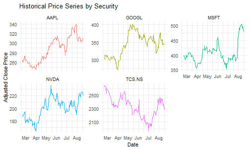

plot of chunk recipe-2-faceted-plot

3. Intraday Price Series & Timeframes

Retrieve high-frequency intraday candles (1m, 5m, 15m, 60m) to examine intraday volatility, liquidity patterns, and trading microstructure.

intraday_5m <- yf_download_prices(
  tickers  = "MSFT",
  period   = "5d",
  interval = "5m"
)

head(intraday_5m)
#> # A tibble: 6 × 8
#>   symbol date                 open  high   low close adj_close
#>   <chr>  <dttm>              <dbl> <dbl> <dbl> <dbl>     <dbl>
#> 1 MSFT   2026-08-12 13:30:00  500.  502.  497.  498.      498.
#> 2 MSFT   2026-08-12 13:35:00  498.  500.  498.  499.      499.
#> 3 MSFT   2026-08-12 13:40:00  499.  499.  497.  498.      498.
#> 4 MSFT   2026-08-12 13:45:00  498.  498.  496.  497.      497.
#> 5 MSFT   2026-08-12 13:50:00  497.  497.  494.  494.      494.
#> 6 MSFT   2026-08-12 13:55:00  494.  494   493.  494.      494.
#> # ℹ 1 more variable: volume <dbl>

Variations & Tips

Hourly Candle Tracking: Download 1-hour candles over the past month:

intraday_1h <- yf_download_prices(
  tickers  = "MSFT",
  period   = "1mo",
  interval = "60m"
)

Intraday Volume Distribution: Visualize intraday trading volume bars:

ggplot(intraday_5m, aes(x = date, y = volume)) +
  geom_col(fill = "#4f46e5", alpha = 0.8) +
  scale_y_continuous(labels = label_number(scale_cut = cut_short_scale())) +
  labs(
    title = "MSFT 5-Minute Intraday Volume",
    x     = "Timestamp (UTC)",
    y     = "Volume"
  ) +
  theme_minimal()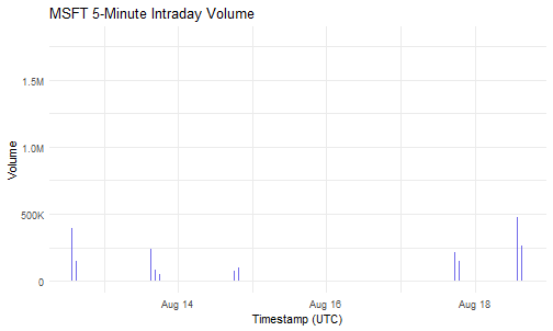

plot of chunk recipe-3-volume-plot

4. Real-Time Market Overview & Regional Filtering

Retrieve live market snapshots across international equity indices, currencies, and commodities, then filter for specific regional exchanges.

market_overview <- get_market_summary(as_tibble = TRUE)

# Filter for Indian indices and INR currency pairs
indian_market <- market_overview |>
  filter(grepl("NSE|BSE|NIFTY|SENSEX|INR", short_name, ignore.case = TRUE))

print(indian_market)
#> # A tibble: 0 × 9
#> # ℹ 9 variables: symbol <chr>, short_name <chr>,
#> #   regular_market_price <dbl>, regular_market_change <dbl>,
#> #   regular_market_change_percent <dbl>,
#> #   regular_market_previous_close <dbl>, market_state <chr>,
#> #   exchange <chr>, market_time <dttm>

Variations & Tips

Filter for Commodities & Crypto:

commodities_crypto <- market_overview |>
  filter(grepl("Gold|Crude|Silver|BTC|ETH", short_name, ignore.case = TRUE))

Alternative Filtering with stringr:

library(stringr)

european_market <- market_overview |>
  filter(str_detect(short_name, regex("DAX|FTSE|CAC", ignore_case = TRUE)))

5. Download Benchmark Index History

Retrieve historical price series for major benchmark indices (^GSPC, ^IXIC, ^NSEI, ^BSESN) and normalize prices to a common base of 100 for comparative performance tracking.

benchmark_symbols <- c("^GSPC", "^IXIC", "^NSEI", "^BSESN")

benchmark_prices <- yf_download_prices(
  tickers  = benchmark_symbols,
  period   = "1y",
  interval = "1d"
)

# Normalize price levels (Base = 100)
normalized_indices <- benchmark_prices |>
  group_by(symbol) |>
  arrange(date) |>
  mutate(indexed_price = (close / first(close)) * 100) |>
  ungroup()

ggplot(normalized_indices, aes(x = date, y = indexed_price, color = symbol)) +
  geom_line(linewidth = 0.8) +
  labs(
    title = "Global Benchmark Performance (Base = 100)",
    x     = "Date",
    y     = "Normalized Growth",
    color = "Index"
  ) +
  theme_minimal()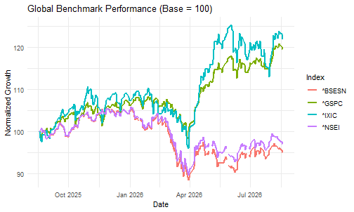

plot of chunk recipe-5-core

Variations & Tips

Indian Sectoral Indices: Track major sector sub-indices:

sectoral_symbols <- c("^CNXIT", "^NSEBANK", "^CNXAUTO")
sectoral_prices  <- yf_download_prices(sectoral_symbols, period = "1y", interval = "1d")

Index Class R6 Query:

nifty <- Index$new("^NSEI")
cat("Index Name:   ", nifty$short_name, "\n")
#> Index Name:
cat("Current Level:", nifty$regular_market_price, "\n")
#> Current Level:

6. Historical Currency & Forex Conversions

Convert foreign asset valuations into a local base currency by retrieving spot and historical foreign exchange rates via ISO 4217 currency pairs.

# 1. Fetch Apple USD prices
aapl <- yf_download_prices("AAPL", period = "6mo") |>
  mutate(date_day = as.Date(date))

# 2. Fetch USD/INR exchange rates
usd_inr <- currency_converter("USD", "INR", period = "6mo") |>
  mutate(date_day = as.Date(date)) |>
  select(date_day, fx_rate = close)

# 3. Join and compute share price in INR
aapl_inr <- aapl |>
  inner_join(usd_inr, by = "date_day") |>
  mutate(close_inr = close * fx_rate) |>
  select(date_day, close_usd = close, fx_rate, close_inr)

head(aapl_inr)
#> # A tibble: 6 × 4
#>   date_day   close_usd fx_rate close_inr
#>   <date>         <dbl>   <dbl>     <dbl>
#> 1 2026-02-18      264.    90.6    23957.
#> 2 2026-02-19      261.    90.8    23659.
#> 3 2026-02-20      265.    91.0    24088.
#> 4 2026-02-23      266.    90.7    24150.
#> 5 2026-02-24      272.    91.0    24770.
#> 6 2026-02-25      274.    90.9    24932.

Variations & Tips

Inspect Available ISO Currency Codes:

supported_currencies <- get_currencies()
head(supported_currencies)
#>   short_name          long_name symbol    local_long_name
#> 1        FJD      Fijian Dollar    FJD      Fijian Dollar
#> 2        MXN       Mexican Peso    MXN       Mexican Peso
#> 3        SCR  Seychellois Rupee    SCR  Seychellois Rupee
#> 4        CDF    Congolese Franc    CDF    Congolese Franc
#> 5        GTQ Guatemalan Quetzal    GTQ Guatemalan Quetzal
#> 6        BBD   Barbadian Dollar    BBD   Barbadian Dollar

Direct Forex Pair Download: Query exchange rates using the =X ticker convention:

fx_basket <- yf_download_prices(c("EURUSD=X", "GBPUSD=X", "USDJPY=X"), period = "3mo")

7. Validate Ticker Symbols Before Pipelines

Sanitize, filter, and audit arbitrary universes of ticker symbols prior to running batch download pipelines to prevent failures caused by delisted or malformed symbols.

raw_symbols <- c("AAPL", "INVALID_XYZ", "TCS.NS", "NOT_REAL_123", "MSFT")

# 1. Return valid tickers only
clean_symbols <- validate(raw_symbols)
print(clean_symbols)
#> [1] "AAPL"   "TCS.NS" "MSFT"

# 2. Named logical audit vector
validation_status <- validate(raw_symbols, return_logical = TRUE)
print(validation_status)
#>         AAPL  INVALID_XYZ       TCS.NS NOT_REAL_123         MSFT 
#>         TRUE        FALSE         TRUE        FALSE         TRUE

# 3. Clean inline before download
clean_prices <- yf_download_prices(
  tickers = validate(raw_symbols),
  period  = "3mo"
)

head(clean_prices)
#> # A tibble: 6 × 8
#>   symbol date                 open  high   low close adj_close
#>   <chr>  <dttm>              <dbl> <dbl> <dbl> <dbl>     <dbl>
#> 1 AAPL   2026-05-18 13:30:00  300.  301.  295.  298.      298.
#> 2 AAPL   2026-05-19 13:30:00  297.  301.  296.  299.      299.
#> 3 AAPL   2026-05-20 13:30:00  298.  303.  298.  302.      302.
#> 4 AAPL   2026-05-21 13:30:00  301.  306.  300.  305.      305.
#> 5 AAPL   2026-05-22 13:30:00  306.  311.  306.  309.      309.
#> 6 AAPL   2026-05-26 13:30:00  310.  312.  308.  308.      308.
#> # ℹ 1 more variable: volume <dbl>

Variations & Tips

Audit and Warning Log for Rejected Tickers:

status <- validate(raw_symbols, return_logical = TRUE)
invalid_tickers <- names(status[!status])

if (length(invalid_tickers) > 0) {
  warning("Dropped invalid tickers: ", paste(invalid_tickers, collapse = ", "))
}

8. Calculate Daily Percentage Returns

Calculate simple discrete percentage returns and continuous log returns across multiple securities using standardized adjusted close prices (adj_close).

symbols <- c("AAPL", "MSFT", "GOOGL")

returns_df <- yf_download_prices(symbols, period = "1y", interval = "1d") |>
  group_by(symbol) |>
  arrange(date) |>
  mutate(
    daily_return = (adj_close / lag(adj_close)) - 1,
    log_return   = log(adj_close / lag(adj_close))
  ) |>
  filter(!is.na(daily_return)) |>
  ungroup()

head(returns_df)
#> # A tibble: 6 × 10
#>   symbol date                 open  high   low close adj_close
#>   <chr>  <dttm>              <dbl> <dbl> <dbl> <dbl>     <dbl>
#> 1 AAPL   2025-08-19 13:30:00  231.  233.  229.  231.      230.
#> 2 MSFT   2025-08-19 13:30:00  515   515.  509.  510.      506.
#> 3 GOOGL  2025-08-19 13:30:00  203.  203.  200.  202.      201.
#> 4 AAPL   2025-08-20 13:30:00  230.  230.  226.  226.      225.
#> 5 MSFT   2025-08-20 13:30:00  510.  511   504.  506.      502.
#> 6 GOOGL  2025-08-20 13:30:00  201.  201.  197.  199.      199.
#> # ℹ 3 more variables: volume <dbl>, daily_return <dbl>,
#> #   log_return <dbl>

Variations & Tips

Visualizing Return Distributions: Plot overlapping density curves to evaluate return dispersion and tail thickness:

ggplot(returns_df, aes(x = daily_return, fill = symbol)) +
  geom_density(alpha = 0.4) +
  scale_x_continuous(labels = label_percent(accuracy = 0.1)) +
  labs(
    title = "Daily Return Distributions",
    x     = "Daily Percentage Return",
    y     = "Density",
    fill  = "Ticker"
  ) +
  theme_minimal()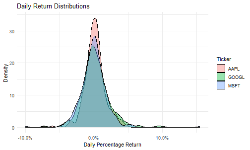

plot of chunk recipe-8-density-plot

Summary Statistics Table:

returns_summary <- returns_df |>
  group_by(symbol) |>
  summarise(
    trading_days  = n(),
    mean_daily    = mean(daily_return),
    sd_daily      = sd(daily_return),
    annual_return = mean_daily * 252,
    annual_vol    = sd_daily * sqrt(252)
  )
print(returns_summary)
#> # A tibble: 3 × 6
#>   symbol trading_days mean_daily sd_daily annual_return annual_vol
#>   <chr>         <int>      <dbl>    <dbl>         <dbl>      <dbl>
#> 1 AAPL            251  0.00131     0.0157        0.329       0.250
#> 2 GOOGL           251  0.00230     0.0206        0.580       0.328
#> 3 MSFT            251 -0.0000526   0.0203       -0.0133      0.323

9. Multi-Asset Return Correlation Matrix

Reshape multi-asset return series into a wide format to compute pairwise Pearson correlation coefficients, assess sector co-movement, and evaluate diversification benefits.

symbols <- c("AAPL", "MSFT", "NVDA", "GLD", "^GSPC")

prices <- yf_download_prices(symbols, period = "1y", interval = "1d")

returns_matrix <- prices |>
  group_by(symbol) |>
  arrange(date) |>
  mutate(daily_return = (adj_close / lag(adj_close)) - 1) |>
  filter(!is.na(daily_return)) |>
  ungroup() |>
  select(date, symbol, daily_return) |>
  pivot_wider(names_from = symbol, values_from = daily_return) |>
  select(-date)

cor_matrix <- cor(returns_matrix, use = "pairwise.complete.obs")
round(cor_matrix, 2)
#>       AAPL MSFT NVDA  GLD ^GSPC
#> AAPL  1.00 0.11 0.12 0.08  0.38
#> MSFT  0.11 1.00 0.27 0.08  0.39
#> NVDA  0.12 0.27 1.00 0.23  0.66
#> GLD   0.08 0.08 0.23 1.00  0.32
#> ^GSPC 0.38 0.39 0.66 0.32  1.00

Variations & Tips

Correlation Heatmap: Visualize asset correlation tiles using ggplot2:

cor_long <- as.data.frame(cor_matrix) |>
  mutate(asset1 = rownames(cor_matrix)) |>
  pivot_longer(-asset1, names_to = "asset2", values_to = "correlation")

ggplot(cor_long, aes(x = asset1, y = asset2, fill = correlation)) +
  geom_tile(color = "white") +
  geom_text(aes(label = round(correlation, 2)), color = "black", size = 4) +
  scale_fill_gradient2(
    low = "#d73027", mid = "#ffffbf", high = "#1a9850",
    midpoint = 0, limit = c(-1, 1), name = "Correlation"
  ) +
  labs(title = "Asset Return Correlation Matrix", x = NULL, y = NULL) +
  theme_minimal()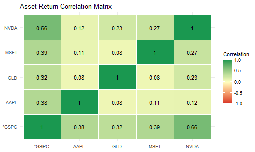

plot of chunk recipe-9-heatmap

Rolling 60-Day Pairwise Correlation: Track correlation stability over time:

rolling_cor <- returns_matrix |>
  mutate(
    roll_cor_aapl_gspc = rollapplyr(
      data      = cbind(AAPL, `^GSPC`),
      width     = 60,
      FUN       = function(x) cor(x[, 1], x[, 2], use = "complete.obs"),
      by.column = FALSE,
      fill      = NA
    )
  )

10. Compute Moving Averages & Trend Crossovers

Calculate 50-day and 200-day Simple Moving Averages (SMA) to classify market trend regimes and detect Golden Cross and Death Cross crossover signals.

prices <- yf_download_prices("AAPL", period = "2y", interval = "1d")

sma_df <- prices |>
  arrange(date) |>
  mutate(
    sma_50  = rollmeanr(adj_close, k = 50, fill = NA),
    sma_200 = rollmeanr(adj_close, k = 200, fill = NA),
    regime  = case_when(
      sma_50 > sma_200 ~ "Bullish (SMA50 > SMA200)",
      sma_50 < sma_200 ~ "Bearish (SMA50 < SMA200)",
      TRUE             ~ "Neutral"
    ),
    signal  = case_when(
      sma_50 > sma_200 & lag(sma_50) <= lag(sma_200) ~ "Golden Cross",
      sma_50 < sma_200 & lag(sma_50) >= lag(sma_200) ~ "Death Cross",
      TRUE                                           ~ NA_character_
    )
  )

tail(sma_df |> select(date, close, adj_close, sma_50, sma_200, regime, signal), 6)
#> # A tibble: 6 × 7
#>   date                close adj_close sma_50 sma_200 regime  signal
#>   <dttm>              <dbl>     <dbl>  <dbl>   <dbl> <chr>   <chr> 
#> 1 2026-08-11 13:30:00  305.      305.   309.    279. Bullis… <NA>  
#> 2 2026-08-12 13:30:00  302.      302.   309.    280. Bullis… <NA>  
#> 3 2026-08-13 13:30:00  305.      305.   309.    280. Bullis… <NA>  
#> 4 2026-08-14 13:30:00  306.      306.   309.    280. Bullis… <NA>  
#> 5 2026-08-17 13:30:00  306.      306.   309.    280. Bullis… <NA>  
#> 6 2026-08-18 13:30:00  310.      310.   309.    280. Bullis… <NA>

Variations & Tips

Moving Average Overlay Chart:

ggplot(filter(sma_df, !is.na(sma_200)), aes(x = date)) +
  geom_line(aes(y = adj_close), color = "gray60", alpha = 0.7, linewidth = 0.5) +
  geom_line(aes(y = sma_50, color = "50-day SMA"), linewidth = 0.9) +
  geom_line(aes(y = sma_200, color = "200-day SMA"), linewidth = 0.9) +
  scale_color_manual(
    name   = "Indicators",
    values = c("50-day SMA" = "#1f77b4", "200-day SMA" = "#d62728")
  ) +
  labs(
    title    = "AAPL Price Trend & Moving Averages",
    subtitle = "50-Day vs. 200-Day Simple Moving Average",
    x        = "Date",
    y        = "Adjusted Price (USD)"
  ) +
  theme_minimal() +
  theme(legend.position = "bottom")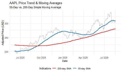

plot of chunk recipe-10-ma-chart

Exponential Moving Average (EMA): Weight recent observations higher:

alpha <- 2 / (20 + 1)
sma_df <- sma_df |>
  mutate(ema_20 = stats::filter(adj_close * alpha, 1 - alpha, method = "recursive", sides = 1))

11. Calculate Historical & Maximum Drawdown (MDD)

Compute running peak prices and peak-to-trough percentage drawdowns to quantify historical capital loss risk, tail risk, and maximum drawdown limits.

prices <- yf_download_prices("NVDA", period = "5y", interval = "1d")

drawdown_df <- prices |>
  arrange(date) |>
  mutate(
    peak_price = cummax(adj_close),
    drawdown   = (adj_close - peak_price) / peak_price
  )

max_dd_val <- min(drawdown_df$drawdown, na.rm = TRUE)
worst_row  <- drawdown_df |> filter(drawdown == max_dd_val) |> slice(1)

cat("Maximum Drawdown (MDD):", sprintf("%.2f%%", max_dd_val * 100), "\n")
#> Maximum Drawdown (MDD): -66.34%
cat("Trough Date:           ", format(worst_row$date, "%Y-%m-%d"), "\n")
#> Trough Date:            2022-10-14
cat("Trough Price:          ", round(worst_row$adj_close, 2), "\n")
#> Trough Price:           11.2
cat("Previous Peak Price:   ", round(worst_row$peak_price, 2), "\n")
#> Previous Peak Price:    33.27

Variations & Tips

Underwater Area Chart:

ggplot(drawdown_df, aes(x = date, y = drawdown)) +
  geom_area(fill = "#d9534f", alpha = 0.4) +
  geom_line(color = "#d9534f", linewidth = 0.7) +
  scale_y_continuous(labels = label_percent()) +
  labs(
    title    = "NVDA Historical Drawdown (Underwater Chart)",
    subtitle = paste0("Max Drawdown: ", sprintf("%.2f%%", max_dd_val * 100)),
    x        = "Date",
    y        = "Drawdown from Peak"
  ) +
  theme_minimal()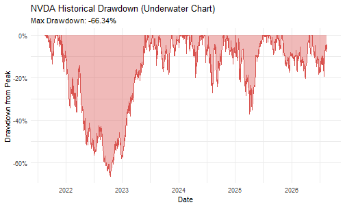

plot of chunk recipe-11-underwater-chart

Multi-Asset MDD Comparison: Compare worst-case drawdowns across securities:

multi_basket <- yf_download_prices(c("AAPL", "MSFT", "GOOGL", "^GSPC"), period = "5y")

mdd_comparison <- multi_basket |>
  group_by(symbol) |>
  arrange(date) |>
  mutate(
    peak = cummax(adj_close),
    dd   = (adj_close - peak) / peak
  ) |>
  summarise(
    max_drawdown     = min(dd, na.rm = TRUE),
    current_drawdown = last(dd)
  ) |>
  arrange(max_drawdown)

print(mdd_comparison)
#> # A tibble: 4 × 3
#>   symbol max_drawdown current_drawdown
#>   <chr>         <dbl>            <dbl>
#> 1 GOOGL        -0.443          -0.148 
#> 2 MSFT         -0.371          -0.106 
#> 3 AAPL         -0.334          -0.0890
#> 4 ^GSPC        -0.254          -0.0123

12. Calculate Stock Beta & CAPM Alpha

Fit a Capital Asset Pricing Model (CAPM) linear regression against a broad market index to estimate systematic market risk ( $\beta$ ) and abnormal alpha ( $\alpha$ ).

prices <- yf_download_prices(c("AAPL", "^GSPC"), period = "2y", interval = "1d")

returns_wide <- prices |>
  group_by(symbol) |>
  arrange(date) |>
  mutate(daily_return = (adj_close / lag(adj_close)) - 1) |>
  filter(!is.na(daily_return)) |>
  ungroup() |>
  select(date, symbol, daily_return) |>
  pivot_wider(names_from = symbol, values_from = daily_return) |>
  drop_na()

capm_fit <- lm(AAPL ~ `^GSPC`, data = returns_wide)
fit_summary <- summary(capm_fit)

alpha_daily <- coef(capm_fit)[1]
beta        <- coef(capm_fit)[2]
r_squared   <- fit_summary$r.squared

cat("Beta (Systematic Risk):", round(beta, 3), "\n")
#> Beta (Systematic Risk): 1.108
cat("Daily Alpha:           ", sprintf("%.4f%%", alpha_daily * 100), "\n")
#> Daily Alpha:            0.0049%
cat("Annualized Alpha:      ", sprintf("%.2f%%", alpha_daily * 252 * 100), "\n")
#> Annualized Alpha:       1.23%
cat("R-Squared:             ", round(r_squared, 3), "\n")
#> R-Squared:              0.391

Variations & Tips

CAPM Regression Scatter Plot:

ggplot(returns_wide, aes(x = `^GSPC`, y = AAPL)) +
  geom_point(alpha = 0.4, color = "#2c3e50") +
  geom_smooth(method = "lm", color = "#e74c3c", se = TRUE) +
  scale_x_continuous(labels = label_percent()) +
  scale_y_continuous(labels = label_percent()) +
  labs(
    title    = "AAPL vs. S&P 500 (CAPM Beta Regression)",
    subtitle = paste0("Beta = ", round(beta, 2), " | R² = ", round(r_squared, 2)),
    x        = "S&P 500 Daily Return",
    y        = "AAPL Daily Return"
  ) +
  theme_minimal()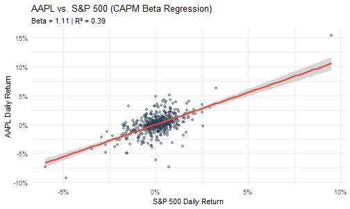

plot of chunk recipe-12-regression-plot

Batch Beta Calculation for Indian Stocks:

in_basket  <- c("TCS.NS", "INFY.NS", "RELIANCE.NS", "HDFCBANK.NS", "^NSEI")
in_prices  <- yf_download_prices(in_basket, period = "2y", interval = "1d")

in_returns <- in_prices |>
  group_by(symbol) |>
  arrange(date) |>
  mutate(ret = (adj_close / lag(adj_close)) - 1) |>
  filter(!is.na(ret)) |>
  ungroup() |>
  select(date, symbol, ret) |>
  pivot_wider(names_from = symbol, values_from = ret) |>
  drop_na()

stocks <- setdiff(names(in_returns), c("date", "^NSEI"))
beta_table <- tibble(
  symbol = stocks,
  beta   = sapply(stocks, function(s) cov(in_returns[[s]], in_returns[["^NSEI"]]) / var(in_returns[["^NSEI"]]))
) |> arrange(desc(beta))

print(beta_table)
#> # A tibble: 4 × 2
#>   symbol       beta
#>   <chr>       <dbl>
#> 1 HDFCBANK.NS 1.08 
#> 2 RELIANCE.NS 1.04 
#> 3 INFY.NS     0.924
#> 4 TCS.NS      0.845

13. Portfolio Cumulative Returns & Wealth Index (Growth of $10,000)

Simulate a multi-asset portfolio, compound daily percentage returns over time, and compare the growth of a hypothetical $10,000 investment against the S&P 500 index.

tickers <- c("AAPL", "MSFT", "NVDA", "^GSPC")

prices <- yf_download_prices(tickers, period = "2y", interval = "1d")

returns_df <- prices |>
  group_by(symbol) |>
  arrange(date) |>
  mutate(daily_return = (adj_close / lag(adj_close)) - 1) |>
  filter(!is.na(daily_return)) |>
  ungroup()

# Equal-weighted tech basket
portfolio_returns <- returns_df |>
  filter(symbol != "^GSPC") |>
  group_by(date) |>
  summarise(daily_return = mean(daily_return), .groups = "drop") |>
  mutate(symbol = "Equal-Weight Tech Portfolio")

benchmark_returns <- returns_df |>
  filter(symbol == "^GSPC") |>
  select(date, symbol, daily_return)

wealth_df <- bind_rows(portfolio_returns, benchmark_returns) |>
  group_by(symbol) |>
  arrange(date) |>
  mutate(
    cum_return   = cumprod(1 + daily_return) - 1,
    wealth_index = 10000 * cumprod(1 + daily_return)
  ) |>
  ungroup()

wealth_df |>
  group_by(symbol) |>
  slice_tail(n = 1) |>
  select(symbol, date, cum_return, wealth_index)
#> # A tibble: 2 × 4
#> # Groups:   symbol [2]
#>   symbol                date                cum_return wealth_index
#>   <chr>                 <dttm>                   <dbl>        <dbl>
#> 1 Equal-Weight Tech Po… 2026-08-18 13:30:00      0.471       14715.
#> 2 ^GSPC                 2026-08-18 13:30:00      0.373       13735.

Variations & Tips

Growth of $10,000 Visualization:

ggplot(wealth_df, aes(x = date, y = wealth_index, color = symbol)) +
  geom_line(linewidth = 0.9) +
  scale_y_continuous(labels = label_dollar(prefix = "$")) +
  labs(
    title = "Growth of $10,000: Tech Portfolio vs. S&P 500",
    x     = "Date",
    y     = "Portfolio Value ($)",
    color = "Strategy"
  ) +
  theme_minimal() +
  theme(legend.position = "bottom")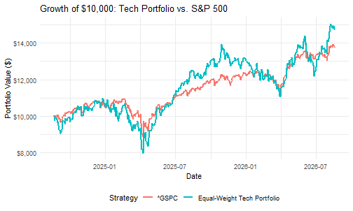

plot of chunk recipe-13-wealth-plot

Custom Asset Allocation Weights:

weights <- c("NVDA" = 0.50, "AAPL" = 0.30, "MSFT" = 0.20)

custom_port <- returns_df |>
  filter(symbol %in% names(weights)) |>
  mutate(weight = weights[symbol]) |>
  group_by(date) |>
  summarise(daily_return = sum(daily_return * weight), .groups = "drop") |>
  mutate(
    cum_return   = cumprod(1 + daily_return) - 1,
    wealth_index = 10000 * cumprod(1 + daily_return)
  )

14. Calculate Sharpe Ratio & Risk-Adjusted Metrics

Evaluate asset risk efficiency by computing annualized return, volatility, downside deviation, the Sharpe Ratio, and the Sortino Ratio relative to a risk-free benchmark rate ( $R_f$ ).

prices <- yf_download_prices(c("AAPL", "MSFT", "NVDA", "^GSPC"), period = "2y", interval = "1d")

rf_annual <- 0.04
rf_daily  <- rf_annual / 252

performance_metrics <- prices |>
  group_by(symbol) |>
  arrange(date) |>
  mutate(
    daily_return  = (adj_close / lag(adj_close)) - 1,
    excess_return = daily_return - rf_daily
  ) |>
  filter(!is.na(daily_return)) |>
  summarise(
    trading_days      = n(),
    annual_return     = mean(daily_return) * 252,
    annual_volatility = sd(daily_return) * sqrt(252),
    sharpe_ratio      = (annual_return - rf_annual) / annual_volatility,
    downside_vol      = sqrt(mean(pmin(excess_return, 0)^2)) * sqrt(252),
    sortino_ratio     = (annual_return - rf_annual) / downside_vol,
    .groups           = "drop"
  ) |>
  arrange(desc(sharpe_ratio))

print(performance_metrics)
#> # A tibble: 4 × 7
#>   symbol trading_days annual_return annual_volatility sharpe_ratio
#>   <chr>         <int>         <dbl>             <dbl>        <dbl>
#> 1 ^GSPC           500         0.173             0.162        0.820
#> 2 NVDA            500         0.368             0.451        0.727
#> 3 AAPL            500         0.204             0.288        0.570
#> 4 MSFT            500         0.115             0.288        0.259
#> # ℹ 2 more variables: downside_vol <dbl>, sortino_ratio <dbl>

Variations & Tips

Risk vs. Return Bubble Chart:

ggplot(performance_metrics, aes(x = annual_volatility, y = annual_return, color = symbol)) +
  geom_point(aes(size = sharpe_ratio), alpha = 0.8) +
  geom_text(aes(label = symbol), vjust = -1.2, fontface = "bold") +
  geom_hline(yintercept = rf_annual, linetype = "dashed", color = "gray50") +
  scale_x_continuous(labels = label_percent()) +
  scale_y_continuous(labels = label_percent()) +
  scale_size_continuous(range = c(4, 10), name = "Sharpe Ratio") +
  labs(
    title    = "Risk vs. Return Profile",
    subtitle = "Bubble size represents Sharpe Ratio",
    x        = "Annualized Risk / Volatility",
    y        = "Annualized Return"
  ) +
  theme_minimal() +
  theme(legend.position = "right")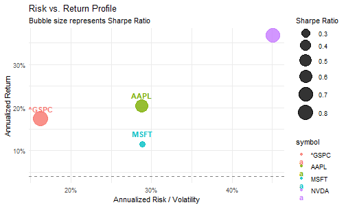

plot of chunk recipe-14-bubble-plot

15. Compute Bollinger Bands & Volatility Envelopes

Construct 20-day volatility envelopes ( $\text{SMA}_{20} \pm 2\sigma$ ), compute $\%B$ and Bandwidth indicators, and screen a universe of stocks for volatility breakouts.

# 1. Download prices for a single security
prices <- yf_download_prices("MSFT", period = "1y", interval = "1d")

# 2. Compute Bollinger Bands, %B, and Bandwidth
bb_df <- prices |>
  filter(!is.na(adj_close)) |>
  arrange(date) |>
  mutate(
    bb_middle = rollmeanr(adj_close, k = 20, fill = NA),
    bb_sd     = rollapplyr(adj_close, width = 20, FUN = sd, fill = NA),
    bb_upper  = bb_middle + (2 * bb_sd),
    bb_lower  = bb_middle - (2 * bb_sd),
    bb_pct_b  = (adj_close - bb_lower) / (bb_upper - bb_lower),
    bandwidth = (bb_upper - bb_lower) / bb_middle
  )

tail(bb_df |> select(date, adj_close, bb_lower, bb_middle, bb_upper, bb_pct_b, bandwidth), 6)
#> # A tibble: 6 × 7
#>   date                adj_close bb_lower bb_middle bb_upper
#>   <dttm>                  <dbl>    <dbl>     <dbl>    <dbl>
#> 1 2026-08-11 13:30:00      504.     334.      436.     537.
#> 2 2026-08-12 13:30:00      492.     338.      440.     543.
#> 3 2026-08-13 13:30:00      497.     342.      445.     549.
#> 4 2026-08-14 13:30:00      495.     347.      450.     553.
#> 5 2026-08-17 13:30:00      480.     353.      454.     555.
#> 6 2026-08-18 13:30:00      481.     360.      458.     557.
#> # ℹ 2 more variables: bb_pct_b <dbl>, bandwidth <dbl>

Variations & Tips

Bollinger Bands Ribbon Plot:

ggplot(filter(bb_df, !is.na(bb_upper)), aes(x = date)) +
  geom_ribbon(aes(ymin = bb_lower, ymax = bb_upper), fill = "#e0e7ff", alpha = 0.6) +
  geom_line(aes(y = bb_upper), color = "#4f46e5", linetype = "dashed", linewidth = 0.5) +
  geom_line(aes(y = bb_middle), color = "#3b82f6", linewidth = 0.8) +
  geom_line(aes(y = bb_lower), color = "#4f46e5", linetype = "dashed", linewidth = 0.5) +
  geom_line(aes(y = adj_close), color = "#1e293b", linewidth = 0.7) +
  labs(
    title    = "MSFT Price with 20-Day Bollinger Bands (±2σ)",
    subtitle = "Shaded channel represents standard volatility envelope",
    x        = "Date",
    y        = "Adjusted Price (USD)"
  ) +
  theme_minimal()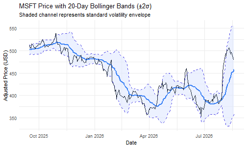

plot of chunk recipe-15-ribbon-plot

Multi-Ticker Volatility Breakout Screener:

watchlist <- c("AAPL", "MSFT", "NVDA", "GOOGL", "AMZN")

screener_results <- yf_download_prices(watchlist, period = "6mo", interval = "1d") |>
  filter(!is.na(adj_close) & !is.na(close)) |>
  group_by(symbol) |>
  arrange(date, .by_group = TRUE) |>
  mutate(
    mb    = rollmeanr(adj_close, k = 20, fill = NA),
    sd    = rollapplyr(adj_close, width = 20, FUN = sd, fill = NA),
    ub    = mb + (2 * sd),
    lb    = mb - (2 * sd),
    pct_b = (adj_close - lb) / (ub - lb)
  ) |>
  filter(!is.na(pct_b)) |>
  slice_tail(n = 1) |>
  ungroup() |>
  mutate(
    status = case_when(
      pct_b > 1.0 ~ "Above Upper Band (Overbought/Breakout)",
      pct_b < 0.0 ~ "Below Lower Band (Oversold/Breakdown)",
      TRUE        ~ "Within Normal Bands"
    )
  ) |>
  select(symbol, date, close = adj_close, ub, lb, pct_b, status)

print(screener_results)
#> # A tibble: 5 × 7
#>   symbol date                close    ub    lb pct_b status        
#>   <chr>  <dttm>              <dbl> <dbl> <dbl> <dbl> <chr>         
#> 1 AAPL   2026-08-18 13:30:00  310.  342.  290. 0.371 Within Normal…
#> 2 AMZN   2026-08-18 13:30:00  260.  296.  219. 0.535 Within Normal…
#> 3 GOOGL  2026-08-18 13:30:00  343.  377.  314. 0.455 Within Normal…
#> 4 MSFT   2026-08-18 13:30:00  481.  557.  360. 0.617 Within Normal…
#> 5 NVDA   2026-08-18 13:30:00  220.  235.  189. 0.672 Within Normal…